Spectral Graph Theory and Segmentation

Motivation

Spectral Graph Theory is a powerful tool as it sits at the center of multiple representation.

• Connects to Graph and manifold, and linear algrbra.
• It’s related to dynamics on graph, related to Markov chain, random walk (diffusion.)
• Could be applied to any point cloud: images, meshes are suited.
• Could be used to perform clustering, segmentation etc.

Linear Algebra Review

There are several ways to see a eigenvalue problem

• $Ax=\lambda x$ Can be seen as finding the invariant subspace and its scaling in a linear transformation.
• $\det(A-\lambda I)=0$ Solution to the eigen polynomial. This defines the algebraic distribution of eigenvalues. Many properties could be derived from it.
• $\max {x^TAx\over x^Tx}$ Can be seen as solution to this optimization problem. Stationary points are eigen values. Maximum and minimum correspond to maximal and minimal eigen value.

Spectral Graph theory is just using this 3rd view, how can we relax the hard combinatorial segmentation problem into some convex easy to solve optimization problem.

Graph Theory

Given a graph $\mathcal V,\mathcal E$ , a adjacency matrix $A$ could be defined. If the graph is un-directed, then the matrix is real symmetric. Thus a $n$ node graph will have $n$ eigenvalues and $n$ eigen vectors.

Below I’ll discuss Laplacian matrix majorly, but here I’ll point out a few application of the adjacency matrix $A$.

• Eigen vector of $A$ is used in PageRank algorithm. As only the eigenvector of the largest eigen value will be all positive, the entries in that vector is defined as eigen centrality. (importance of a node to a network)
• $A$ could be normalized to be the transition matrix of a random walk on graph.

Graph Laplacian and Physics

Then the graph Laplacian could be defined as $L=D-A$ while $D=diag(d_i)=diag(\sum_jA_{ij})$

• It’s positive semi-definite and symmetric
• have $n$ non-negative eigen values.

$L$ could be understood as operator on functions on graph. For a value vector $x$, the action of $L$ on the vector is $Lx=Dx-Ax\\ Lx(i)=\sum_j L_{ij}x_j=d_i x_i-\sum_j A_{ij}x_j=\sum_j A_{ij}(x_i-x_j)$ In the binary network case $Lx(i)=\sum_j L_{ij}x_j=\sum_{j\in N(i)}(x_i-x_j)$ Physically, if you think of $A$ as the conductance in an electric or water pipe network, then $Lx(i)$ is the outward flow from node $i$, when you apply the potential $x$ at each node. So pictorially, we can understood it as diffusivity vector. Thus we can write the dynamics of flow on the network as $\frac {dv}{dt}=Lv=(D-A)v$ Besides, from a static view point the construct $x^TLx$ defines a kind of strain or potential energy $E(x)$ for a network $A$ given the potential $x$. And the flow defined above is just the gradient descent flow of this potential. Mechanically, it’s embedding the graph in a 1d line, giving each node a coordinate $x(i)$, and $E(x)$ is the energy of this configuration, given the weight $A$ as the strength of spring $k_{ij}$.¹

$$x^TLx=\sum_{ij} x_iL_{ij}x_j\\ =\sum_{i,j\in E}x_iA_{ij}(x_i-x_j)=\sum_{i,j\in E}x_jA_{ij}(x_j-x_i)\\ =\frac 12 \sum_{i,j\in E}A_{ij}(x_i-x_j)^2=E$$

Spectrum of Laplacian

Using these physical models, we could understand the spectrum structure of Laplacian, i.e.

Zero Eigenvalue

• 0 eigen value corresponds to 0 strain, i.e. equipotential across each connected components.
  • Thus the dimension of 0 eigen space is the number of connected components in the graph.
  • Each of those eigen vector is the indicator vector of each component.
• Laplacian of non-connected components are diagonal blocks of a matrix.
  • Spectrum of a non-connected network is a union of each of its connected components.

Fiedler Vector (2nd smallest)

• A small eigen value corresponds to small strain, and small flow.
• For a connected graph, Fiedler value and Fiedler vector correspond to the smallest non-zero eigenvalue.
• Thus it describe the (non-uniform) stationary configuration with the least strain $E(x)$.
• It’s the solution to this minimization problem, which is a convex programming.

$$v_2=\arg\min_v \frac{v^TLv}{v^Tv},\;s.t.\; 1^Tv=0,\;v^Tv\neq0$$

• As eigen vectors are minimizing spring energy, they are really useful in visualizing graph / networks.
  • Using $v_2,v_3$ as coordinates to visualize a graph.
  • More could be used to embed higher dim structure.

Spectral Clustering

Application

• Point cloud could be represented as a network. Nearest neighbor (kNN) could be used. And then spectral graph analysis could be run.
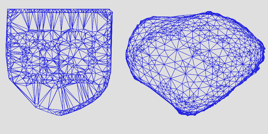
• 3D mesh could be represented as network as well! Weight edge could encode the distance between the nodes. $w_{ij}\propto {|v_i-v_j|^2\over \sigma^2}$

Embedding

Many embedding could be thought of as this energy minimization problem, i.e. stronger spring for points closer by in the cloud, looser or no spring for points farther apart. The only tricky part is how to regularize it

So a typical regularization is this, enforcing each coordinate to be unit variance and orthogonal to each other (no covariance). $\arg\min\sum_{ij}w_{ij}\|f_i-f_j\|^2 ,\; s.t. F^TF=I$ Then, this could be easily optimized by solving the smallest $d$ non-zero eigen vector for the matrix $L$. Note by properties of Laplacian matrix, $F$ will be zero mean automatically. $L_{ij}=w_{ij}\\ LF=\Lambda F$ Then $F_{i,:}$ will be the embedded coordinate for point $i$.

Another choice is using $\Lambda^{-1/2}F$ as coordinate, rescale the embedded axis according to the eigen values! Seems the path length properties will be better.

Clustering

One way of clustering is to do the spectral embedding above, and then do a simple clustering algorithm like k-means in the embedding $d$ space.

So a general spectral clustering algorithm consists of

• Defining a distance (similarity) metric among nodes.
• Use the distance metric to define edge weight, make a graph out of it.
• Compute spectrum of graph laplacian, and the least few eigen vectors.

Segmentation

The most famous work of using graph-cut in computer vision is Shi Malik 2000 . Their major contribution is to modify the objective of the original graph cut, adding a normalization factor, to prevent cutting out too small a piece.

For a 2 segment partitioning problem, the Ncut loss is defined as $Ncut(A,B)=\frac{cut(A,B)}{Ass(A,V)}+\frac{cut(A,B)}{Ass(B,V)}$ After that they find this could be relaxed and solved through a generalized eigenvalue problem.

Computation

These spectral methods all require computation of eigen vector corresponding to small eigen value. It could be performed through Lancosz algorithm. And currently through pre-conditioning method etc. the best performing algorithm is of $O(n)$ complexity of getting that vector.

Reference

See Graph Cut Note for more info.

Spectral Graph Theory Tutorial

spielman Lecture Note

1. Thus solving the minimal energy state for a spring network could be easily done by solving the minimal eigenvalue problem of the Laplacian (with constraint on $|x|$). ↩