
Semantics Vision Task
Note semantics and geometric reasoning is conceptually similar to each other
- Stereo and Optical flow is about finding correspondence / matches.
- Object recognition in some sense is finding correspondence w.r.t. a template, and make the template match the observation.
Semantic Vision before CNN
So ancient semantic detector works like this
- Finding interesting key points
- You want to make it sparse, make the matching problem easier.
- Need to have non-smooth area,
- Region detectors, make it invariant to physical changes as possible.
Keypoint Detector
To do matching and recognition, what is a good Keypoint Detector?
- Superpixel is not a good candidate
- Shape, boundary, change too much, not invariant across scene.
SIFT
Link to Local Feature Descriptor
Set a few heuristic rules to detect blobs.
Blob Detector
Basically, blob detector could be designed by convolving image with some filters and select local maximum (non-maximum suppression). Could use a Laplacian of Guassian as kernel,
\(K=\nabla^2G(0,\sigma^2)\)
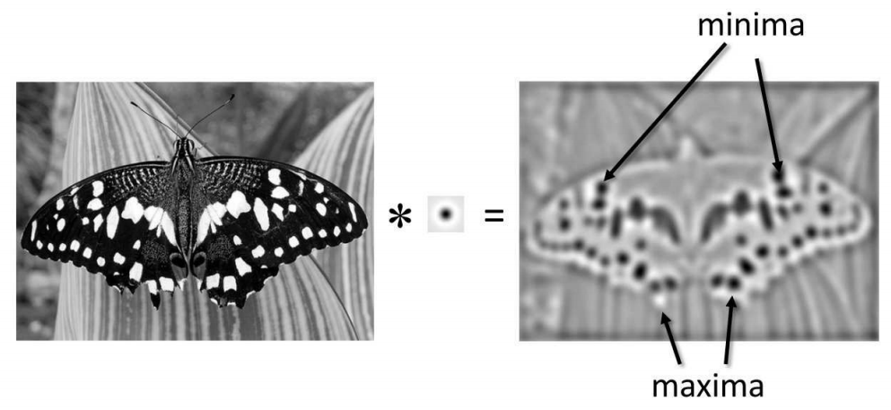
This is the so-called center surround receptive field. (found in many sensory system)
Note:
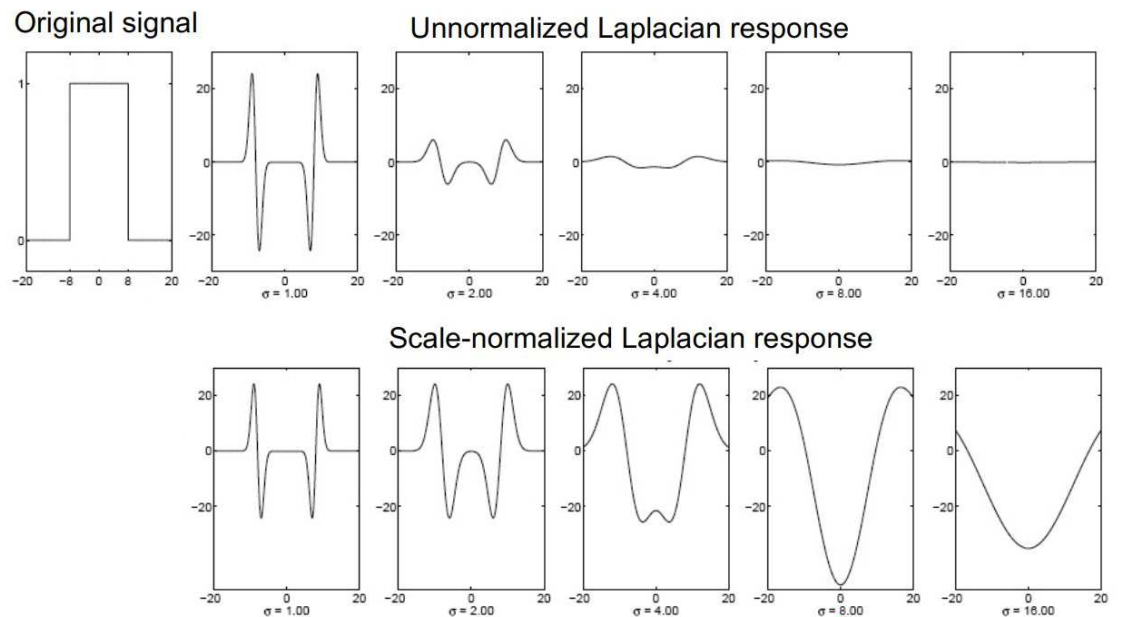
- Only the right size of gaussian $\sigma$ can detect the blob, i.e. you will only detect the blob if the scale matches.
- If the scale doesn’t match, the Laplacian can fire as well! But not give you a single minimum
- So you need to search in scale space!
Scale Space
The observation above gives us the motivation to do the filtering in multiple scales, and detect local maximum in 3d neighborhood.
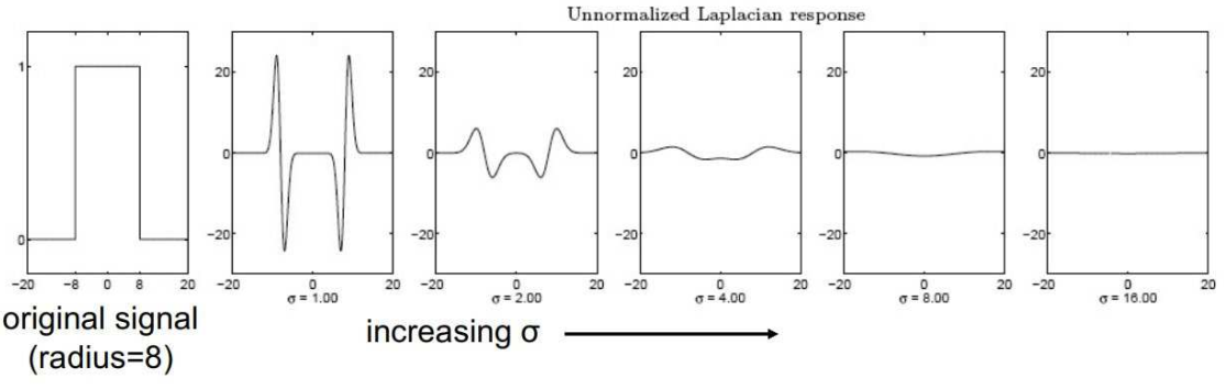
But the higher the $\sigma^2$ the smaller the filter output. Empirically, multiplying $\sigma^2$ factor can renormalize.
\(K = \sigma^2 \nabla^2 G_\sigma\)
Efficiency consideration
Use the Difference of Gaussian (DoG) instead of Laplacian of Gaussian for faster computation (at 2004…), because you can filter image with a pyramid of Gaussians and just take difference between 2 neighbors, to get DoG filtered image. \(K_{DoG} = G(x,y,k\sigma)-G(x,y,\sigma)\)
Suppress Edge
DoG filter will fire at edge as well, have to suppress that.
Compute Hessian of image local patch (Structural Tensor) at the scale of image (Filtered with corresponding $\sigma$ ). And set a criterion that the 2 eigen value of the structural tensor is not very large! Can use tr and det to detect this efficiently.
SIFT Descriptor
Link to Local Feature Descriptor
This are done post hoc, describe the keypoints by a vector to match in this feature space .
Note, ref, Census transform and Hamming distance is the most basic feature descriptor.
Desiderata
- Hope the descriptor to be lighting, scale, rotation invariance
Scale invariance
- Resize the patch to a certain size!
Rotation invariance
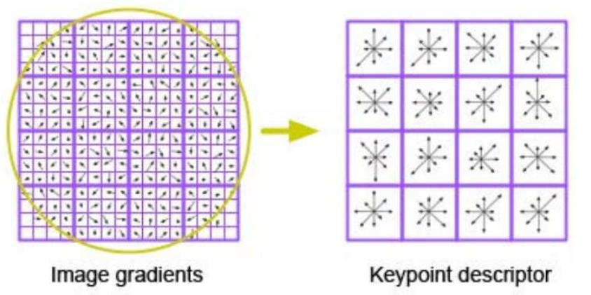
- Do angular histogram for the gradient, find the mode as dominant direction. Then rotate the angle descriptor.
- Pixel is weighted by gradient strength and distance from center to make weighted histogram.
Full SIFT descriptor
- Subdivide region into small non-overlapping regions and concatenate the histogram
Affine Invariance
- Apply affine transformation to the region (not just rotation + scaling) then compute gradient and feature.
Anciently, there is a huge effort to make the better, and evaluate what features should be invariant across view. Things could still be learnt about how features statistics change across view / light
2005 Gradient descent by a bunch of researchers
Mikolajczyk et al., “A Comparison of Affine Region Detectors,” IJCV 2005.
Usage of SIFT
- Even for geometric matching, when you cannot afford to do the dense matching / disparity map, you can do SIFT detection and matching among them.
- Image registration
- SIFT could be used to make a coarse and sparse match!
Content Based Image Retrieval
Note this is quite hard… no one really solve it even now.
Given a query image, find all other images that are “similar”. Thus you need a whole image descriptor to match each other.
2003 ICCV Video Google: Sivic Zisserman
Historical Note: at 2003 NLP is more successful than CV…. so people map semantic vision task to NLP problem for inspiration!
- Step 1: Map SIFT descriptors as “words”
- Do clustering on all SIFTS into discrete labels. Reduce continuous output to discrete
- Note normalized the continuous space by the overall covariance matrix of Descriptor
- Post hoc drop those words that are too frequent or too rare! (Cluster size is too large or too small.)
- Note: this is the same philosophy with the
image atomstudy. Too common or too rare words doesn’t help recognition.
- Note: this is the same philosophy with the
- Step 2: Document images as bag of words, and match image based on occurrence of words.
- Record labels
Building a vocabulary of all possible photographs is hard! (Image Atoms for Object Recognition)
HoG Human Detection
General idea, the keypoint detector and descriptor could be used to solve object recognition problem.
CVPR 2005 Dalal Triggs
Note pedestrian detection and face detection was the only obj detection task at the time…
Basic Thoughts
- Moving a fixed box across image, compute the HoG descriptors
- Use a binary detector to say if it’s a human
- In their case, do HoG on non-overlapping patches in the box,
- Use SVM / perceptron like linear classifier to say if it’s human.
Practise
- Note the binary detector could be applied by convolution the feature tensor for all overlapping patch. (Here its HoG vector.)
- They add local contrastive normalization, normalize a feature by its surround
Comments
- It’s in its essence 1 layer convolutional NN, huge kernel and hand crafted HoG feature descriptor!
- Only classifier is learned, feature extraction is fixed.
- Thus it’s data efficient actually!
- Current CNN is using the Conv Layers to do feature extraction.
Limitation
- This is a single template for an object, doesn’t tolerate deformed spatial structure.
- Note this works for pedestrian and face, as pedestrian and face usually has fixed spatial structure.
Deformable Parts Model
SOTA for a while, inspired modern CNN pooling layer.
2010 PAMI Felzenszwalb, Object detection with Discriminatively Trained Part Based Model
Here we have a graphical model $G=(V,E)$ MRF.
- Vertex is different part of object.
- Cost can be the single part (linear) detector’s prediction.
- Can use HoG feature map and linear detector for each object.
- Edge is the connection between parts.
- Can use a spring cost. Difference between distance and expected distance $|p_i-p_j-(p_{i0}-p_{j0})|$
- You can add a window and upper bound for this spring cost.
Efficiency Note:
- MRF can be inferenced efficiently if it’s a tree!
- We could build a tree like MRF, and a special case star MRF. And the root node can even be an abstract location!
- However, it cannot express all constraints for a physical entity! A general MRF is more expressive but harder to tackle with.
- Efficient inference for this model
- Add a canonical distance / location for each part $(\delta_{x,i},\delta_{y,i})$
To find the best object location root node $p_0$ can be found be maximizing \(S(p_0)=m_0(p_0)+\sum_i \max_{p_i} m_i(p_i)-d_{i0}(p_i,p_0)\) Note :
- The maximization can be very inefficient if $d$ is not structured
- Finally, it’s just convolution (local part detector), moving a window, and maxpooling
- Maxpooling kind of relax the geometric distance constraint of 1 single filter! (“Parts can move now! “)
Training Method
- Latent SVM, train the internal classifiers.
This obsolete model has all the components that a modern CNN has!
- “Hand craft” feature map: SIFT, HoG
- Max pooling: allowing slack relationships between parts
- Learning method: end to end training! No longer latent SVM.
Semantic Vision with CNN
CNN based Object Detection
Taxonomy of Tasks
- Object recognition (classification)
- Segmentation
- Classify pixel based on surrounding patch
- Fully convolutional architecture, diluted convolution, encoder Decoder architecture
- Object detection
Object Detection
The challenge is to propose arbitrary number bounding box with arbitrary shape!
R-CNN
2014 CVPR, Girshick
R-CNN,i.e. region with CNN features
- Propose boxes
- Warp your box
- Pass through
They used MRF based method to do region proposal, Min Cut algorithm.
Constraint Parametric Min Cuts for Automatic Object Segmentation
2015 ICCV, Fast RCNN
- Improve R-CNN to share computation from the start! (R-CNN warp each bounding box so you cannot share convolution)
- You
2015 NIPS, Faster RCNN
- Note, you can have more than one BB centered at each pixel.
- You cannot let one pixel output only one box,
- Non-maxima suppression to reduce redundancy of bounding box.
- Run classifier
YOLO
- First split the image into multiple bounding boxes.
- Each bounding boxes has a bunch of class labels
- Predict property of the box
- 4 coordinates and confidence “objectness”
- Product of objectness $[Math Processing Error]\times$ bounding box label $[Math Processing Error]=$ Final object label.
- Classifier and Box proposal can run in parallel!
Limitation
- There is a strong assumption about object size and grid size!
- Scales dependent! But, you can run multiscale YOLO
- This is super fast, now you can run YOLO real time! Features are real robust!
Object detection is very important, and can be super slow. YOLO change that
Image Segmentation
Segmentation vs Detection
- Detection is able to detect different instances (dog1 bb, dog2 bb, not dogs)
- Segmentation usually just has the class label (this pixel belongs to a “dog” according to surrounding patch).
Image Instance Segmentation
Not just say this pixel is a car, but also label different car instances as different label.
Simplest thought: Combine the Detection and Segmentation,
- Detect the boxes, and do foreground background segmentation within box.
- Graph cut type algorithm could be used.
Neural network version of border distance transform
Distance Transform
- Distance transform find the distance to the closest boundary
- Erode the boundary and find connected components, then you will get different instances
- Assumption is that a instance should be contiguous!
Train a network to produce the distance / watershed transform.
- Distance is not a local entity, hard to know just from local info
- Edge or boundary is local information, thus orientation vector towards boundary is local information.
- You could compute boundary, perform traditional watershed transform $d(I)$, compute gradient $\nabla d(I)$
- These proxy could be used as intermediate supervision.
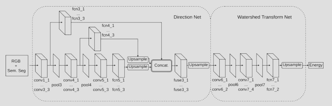
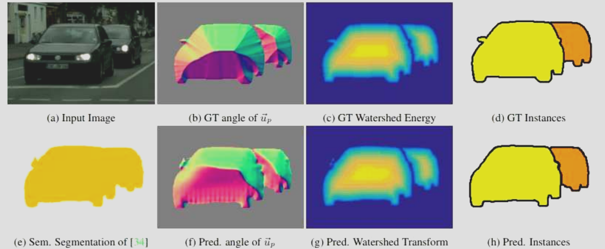
Lesson: Key inspiration is that for some task you don’t have a unique label or output (e.g. instance label is interchangeable, cannot train on that). But you can find a unique proxy output (object boundary and distance to boundary) as supervision!
Image Captioning
Many tasks are assuming the image belongs to certain classes! And classify images to them. Natural language description is one step forward, seeking richer description!
Amusingly finding images and the natural language caption on Internet is not hard! (Semantic data is more abundant than physical or optical data)
NLP 101 : Sequence Generation
Seems not a traditional classification task: (space of sentences is exponentially large! Generative power of language)
But how do you generate these “semi-structured “ output?
- Sequence of words -> Sequence of vectors (can be one-hot encoding. )
- This sequence can be seen as a joint distribution on list of vectors $p([S_1,S_2,S_3…S_n,stop])$, NN can predict the distribution of next word based on the first few words and then recursively generate new words. $p(S_n\mid[S_{1:n-1}])=f([S_{1:n-1}])$
- But the problem of this idea is, you still have different size input for the Next word predictor, which is not map.
- So come the idea of recursive computation and intermediate input, assuming this map is homogeneous (thus recursive).
Intermediate output
- Use RNN to solve this, hope it learns a good intermediate representation, without direct supervision.
- Hope $m_{n-1}$ will be a representation of $S_{1:n-1}$ which is useful for next word prediction
- Since some info in $S_{1:n-1}$ is useful for prediction, some words are not, so Gating is important in these thing.
- Pass a latent representation through (RNN): $p_i,m_i=f(S_{i-1},m_{i-1})$
- $p_i$ is a distribution over words, but $S_{i-1}$ is a specific last word. So you need to choose one!
Practicality: Solving the arbitrary length problem
- Add the word
startstopas marker to start a sentence and stop a statement.
What we need is to prime our sentence generation machine by a image.
Sorry, but CNN representation is not written in English…So need to translate your visual features to the linguistic representation. (A dictionary or embedding links the two.)
- So we need a translation dictionary $(F,D)$ matrix $W$ linearly mapping $D$ dim distribution over words to $F$ dim visual representation.
- The $S_i$ words could be represented in $F$ dim visual feature space. $x_i=WS_i$
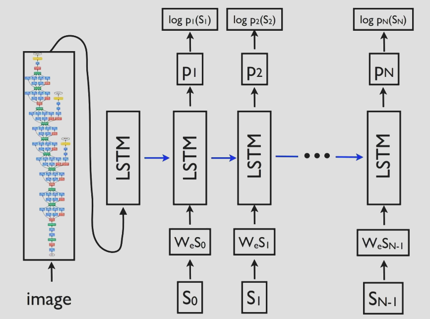
Sequence Model Training
- Use the last word $S_{n-1}$ (correct initial sentence) to predict the current word
- $[p(S_n), m_n]=f(S_{n-1},m_{n-1}(S_{1:n-2};\theta);\theta)$
- $p(S_n)$ can be used to compute loss and gradient.
- Build as deep a network as your output sentence.
- Note you need a different computational graph for different sentences! which requires a eager execution
autogradframework. - Thus,
torchwas much more preferred thantfsincetfrebuilding graph takes so much time!
- Note you need a different computational graph for different sentences! which requires a eager execution
- Mini-Batch: Different length output
- You can batch together sentences output of same length!
- Or you can run several sentences, average the gradient and apply it.
Model Architecture: LSTM
Motivation
- Vanishing / Exploding Gradient is classic problem in RNN
- LSTM designed to address this!
Gating Variable: more refined manipulation of memory vector than linear map.
- $i_i,f_i,o_i$ : input weighting, memory decaying and output weighting variable.
Gated Recurrent Unit (GRU) inherit the gating idea and work as well \(z_{t}=\sigma _{g}(W_{z}x_{t}+U_{z}h_{t-1}+b_{z})\\ r_{t}=\sigma _{g}(W_{r}x_{t}+U_{r}h_{t-1}+b_{r})\\ h_{t}=z_{t}\odot h_{t-1}+(1-z_{t})\odot \phi _{h}(W_{h}x_{t}+U_{h}(r_{t}\odot h_{t-1})+b_{h})\)
- Still one forget gate $z_t$ and one $r_t$ masking last hidden vector
Sequence Model Inference
Inference is trickier than training
- Note this probabilistic language model can generate many different sentences! How do we sample from that?
- Greedy approach : Over committing to one choice at first is not a good idea……(Choose the optimal first word is not optimal at all. Severely suboptimal…)
- Exhaustive Search : The sample number grows too fast. Not practical.
- Beam Search: Each time keep the top-k sentences forward one step through RNN generate D samples. Pick the top k in all the children generation. Iterate
- You can have different length
- It’s kind of a tree search algorithm! Each node can have $D$ children, each time you keep the top $k$ leaves and keep growing from them until termination!
- Note: These sequence model are generative in nature when inference
This kind of problem is common to probabilistic sequence generation! The inference inefficiency of sound generating WaveNet is the same problem!
Evaluation
- Evaluating caption can be done humanly using MTurk, or semantic distance to a real caption!
2015 Neural Image Captioning