Motivation

There is a resurgent of interest in investigating and developing Hopfield network in recent years. This development is quite exciting in that it connect classic models in physics and machine learning to modern techniques like transformers.

Insights from Modern Hopfield Network (Hopfield16)

Energy function is the key for Hopfield network, the update rules follows.

Classic Hopfield network has the energy to minimize. \(E(\xi)=-\xi^TM\xi\) If the connectivity matrix is settled as this
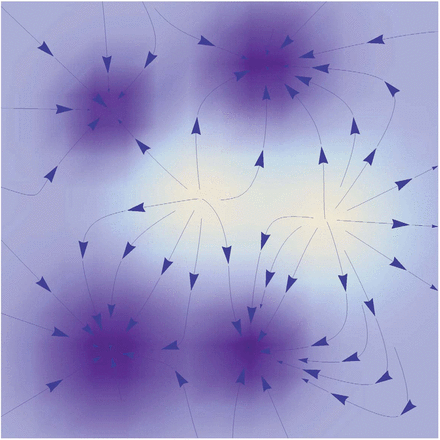
\(M=\sum_i^K x_ix_i^T - I\) Then the Energy function could be rewritten as \(E(\xi)=-\sum_i^K(x_i^T\xi)^2+K\|\xi\|^2\) So In Hopfield16¹, they generalize the quadrative functions to any monotonic function, like Polynomial $x^n$ or rectified polynomial. This choice will shape the energy landscape and finally change the converging: Larger exponent creates a flatter surround and creates higher energy for far apart patterns. \(E(\xi)=-\sum_i^KF(x_i^T\xi)\)

Additionally, they recognized that, there is no real difference between feedforward MLP and recurrent networks.

• If you set part of your recurrent node as layer1, part as layer2, then recurrence between them can be equivalent to feed forward network.
  • E.g.: Hopfield network with 784 node representing pixel, 10 nodes representing numbers.
  • Updating part of the 10 nodes will be equivalent to feedforward pass.
• Fundamentally, in statistical learning, learning a mapping from $x\to y$ and learning the joint distribution of $(x,y)$ is kind of equivalent. You can recover the function or conditional distribution from the joint.

Insights from All you Need2020

In this step they develop the modern Hopfield network to support continuous variables, and find an energy function that link classic methods to transformers.

They designed an energy function using logsumexp with a pattern norm regularization \(E(\xi)=-lse(\beta,X^T\xi)+\|\xi\|^2 + C\\ C = \beta^{-1}\log N+\frac 12M^2,\;\;M=\max_i\|x_i\|\) lse is the process to exponentially transform a vector to positive values and then log transform it back. \(\mbox{lse}(\beta,x)=\beta^{-1}\log(\sum^N_i\exp(\beta x_i))\\ \exp(\beta \mbox{lse}(\beta,x))=\sum^N_i\exp(\beta x_i)\) It’s really connected to softmax function \(\mbox{softmax}(\beta x)_i=\frac{\exp(\beta x_i)}{\sum^N_i\exp(\beta x_i)}=\exp(\beta(x_i-\mbox{lse}(\beta,x)))\) With this energy, they recovered the update rule very similar to transformers. $X$ is of shape $(d,N)$ pattern dimension by number of patterns. \(\xi^{t+1}=X \mbox{sofmax}(\beta X^T\xi^t)\) This update rule has a clear interpretation! Use inner product to find the most similar patterns stored in $X$ and mixing up the most similar patterns using softmax as weight. In a sense, this is the same as retrieving values from $X$ using content $\xi$ as query.

Similarity in Training Philosophy

Hopfield network was known as auto-associative method, which in the neuronal interpretation, each neuron tries to predict its own value by the activations of all other neurons. So in the training process, after looking at each pattern $x_i$, each neuron is required predict its own value in the pattern. $x_i[k]=f(Wx_i)[k]$ . This fixed point equation makes the training works.

• This general concept is similar to the auto-regressive, predict missing pixel process used in training pixel RNN, pixel CNN.

• This is even similar to the missing word prediction scheme used in GPT.

Link to Transformer

This connection is interesting since it bridges so many classic and so many deep methods

• Conceptually similar to vector quantization, K nearest neighbor.

• The convergence process of a RNN like Hopfield network could be regarded as a Feed forward processing layer in neural network.
  • Converging to a single pattern is like one step forward in a feed forward layer.
• Hopfield in its original form is an RNN, and it could be regarded as a feedforward network, and now it’s also transformer.

Reference

The key papers for this development:

1. [1606.01164] Dense Associative Memory for Pattern Recognition Dmitry Krotov, John J Hopfield ↩