
Motivations
Many CNN models have become the bread and butter in modern deep learning pipeline. Here I’m summarizing some famous CNN structure and their key innovations as I use them.
My personal motivation of writing this note is that I’m interested in visual hierarchy in biological and artificial brain. And to investigate the activity and structure in the CNNs, I need a way to listen to the single units or neural populations in it. Thus, I need to understand the “anatomy” of each model and see how that impact the unit property!
ResNet
Here I’m looking at the ResNet101 in torchvision model zoo.
- Core concept of ResNet is to add residue connection in the conv layers which give the feature map a short cut to by pass some conv layer. It will be an identity operator for most layers, and when there is downsampling by strided convolution or
MaxPooling, the residue connection will be adownsampleoperator (by convolution) to match the size of feature map. - The core building block of ResNet is the residue module which can be a
Bottleneckmodule or aBasicBlock.- The
Bottleneckmodule has the following structure, it’s a sandwich of convolution and batch normalization and a ReLU nonlinearity on top of it. It’s a bottleneck in the sense that it shrink the channel dimension of inputs by e.g. 4 fold and then expand back, but may not change the spatial dimensions. (since 1x1 and 3x3 convolutions are used.)
- The
Bottleneck(
    (conv1): Conv2d(1024, 256, kernel_size=(1, 1), stride=(1, 1), bias=False)
    (bn1): BatchNorm2d(256, eps=1e-05, momentum=0.1, affine=True, track_running_stats=True)
    (relu): ReLU(inplace=True)
    (conv2): Conv2d(256, 256, kernel_size=(3, 3), stride=(1, 1), padding=(1, 1), bias=False)
    (bn2): BatchNorm2d(256, eps=1e-05, momentum=0.1, affine=True, track_running_stats=True)
    (relu): ReLU(inplace=True)
    (conv3): Conv2d(256, 1024, kernel_size=(1, 1), stride=(1, 1), bias=False)
    (bn3): BatchNorm2d(1024, eps=1e-05, momentum=0.1, affine=True, track_running_stats=True)
    (relu): ReLU(inplace=True)
)
-
In the
Bottleneckmodule the channel dimension is first reduced by a 1x1 convolution, which is just a feature-wise transformation. Then a batch normalization follows. and a 3x3 convolution follows. Finally a 1x1 convolution expand the channel dimension back to before.-
downsamplepart has an interesting function, it adds a downsampled version of the input to the bottleneck module to the output, and then go through relu. which bypass the Conv and BN layers. This part implement the residue connection.out = self.bn3(out) if self.downsample is not None: identity = self.downsample(x) else: identity = x out += identity out = self.relu(out)
-
- There is a ReLU following each BN layer.
MaxPoolingis used only once at the first part, not in the major bulk of the pipeline.-
AvgPoolingfollowed by reshaping is used just like theAlexNetandVGG - For example
ResNet101has 44549160 parameters, actually this is not a lot. 170Mb on disk.
DenseNet
- The key insight of DenseNet is that, why should we make have a chain like structure in CNNs, where only $L-1$ layer feeds into $L$ layer. We can feed many other previous layers $L-m, L-m+1,…L-1$ into $L$ layer together. That’s the meaning of Dense connection.
- Implementation level, as long as the inputs have the same spatial dimensions, we could concatenate them along the channel dimension and just have a
Conv2dlayer over it, then the $L$ layer will learn to distribute the weights between these layer’s inputs. - It could be thought of as an extension of the Residue connection which feed the $L-d$ layer output into $L$ layer.
- Implementation level, as long as the inputs have the same spatial dimensions, we could concatenate them along the channel dimension and just have a
- The building block of DenseNet is the the
DenseBlockdemonstrated in this code snippet.- It’s a recursive process i.e. do convolution, concatenate the feature maps and do conv on the whole thing again.
class _DenseBlock(nn.ModuleDict):
    _version = 2

    def __init__(self, num_layers, num_input_features, bn_size, growth_rate, drop_rate, memory_efficient=False):
        super(_DenseBlock, self).__init__()
        for i in range(num_layers):
            layer = _DenseLayer(
                num_input_features + i * growth_rate,
                growth_rate=growth_rate,
                bn_size=bn_size,
                drop_rate=drop_rate,
                memory_efficient=memory_efficient,
            )
            self.add_module('denselayer%d' % (i + 1), layer)

    def forward(self, init_features):
        features = [init_features]
        for name, layer in self.items():
            new_features = layer(features)
            features.append(new_features)
        return torch.cat(features, 1)
Actually, DenseNet is relatively light weighted, the DenseNet 169 is only54Mb on disk.
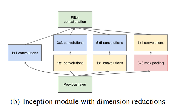
GoogLeNet / Inception Net
In a sense the motivation of Inception module is to reduce computational cost and also go deeper.
- Their solution is to go multi-path, in the same layer, concatenate the result of 1x1, 3x3, 5x5, max-pooling operation along channel dimension.
- Their rationale is, it’s hard to determine the right size of the RF for a neuron, so giving it multiple choices at each level.
- Many technical tricks are used to reduce computational cost.
- In GoogLeNet, 1x1 convolution is used to do channel wise dimension reduction to reduce computational cost.
- Thus a 3x3 conv layer on a high channel dimension tensor is substituted by a 1x1 conv + a 3x3 conv, which reduce the computation and weight.
- V1 has 22 layers, not comparable to ResNet and DenseNet.
- Auxiliary loss for middle layers is used for training purpose.
- Further tricks for efficiency
- 5x5 convolution could be substituted by two 3x3 convolution, i.e. factorization.
- nxn convolution could be substituted by 1xn and nx1 convolution, i.e. factorize the kernel.
- These effectively constrained the larger kernel but also increase efficiency.
-
Further Inception is combined with ResNet to Inception v4.
-
Torch Model GoogLeNet , Inception v3
- Paper GoogLeNet, V1 Going Deeper with Convolution
-
Paper Inception V3 Rethinking the Inception Architecture for Computer Vision
- 10 architecture illustrated